
Transmission Line S-parameters: A Summary and Causality
By ZM Peterson • Jul 7, 2020Although more devices pack more functions into smaller packages, not all devices have shrunk down to smartphone sizes. Devices like servers, backplanes, mainframes, high speed networking equipment, and RF products are ubiquitous outside the consumer electronics market.
These systems are not clearly visible in modern life, but they run behind the scenes and are responsible for making modern life possible. These products all rely on high speed signaling, high frequency wireless or fiber communication, or both. Interconnects in these systems are transmission lines, which require accurate modeling and calculations to describe signal behavior. Some of the mathematical tools required for describing signal behavior are S-parameters, Z-parameters, T-parameters, ABCD parameters, and even the nonlinear X-parameters. Transmission line S-parameters are probably the most important of all these different parameter sets, and they just happen to be the most confusing. Let’s break down the important expressions for S-parameters you’ll need to model signal behavior.
Transmission Line S-parameter Theory
I won’t go too deep into the theory behind S-parameters. Instead, I’ll just summarize the important points behind understanding the most general matrix equation for transmission line S-parameters. In addition, I’ll briefly talk about how this can be used with ABCD parameters for causal modeling of signal behavior in an interconnect.
To get started with transmission line S-parameters, let’s look at the primary model for understanding S-parameters in general for a 2-port network. This is shown in the schematic below. Here, we consider the two basic input signals in the standard S-parameter model for a 2-port network. In addition, we’re assume a linear time-invariant (LTI) system, although we’ll allow nonlinear dispersive behavior in the frequency domain.
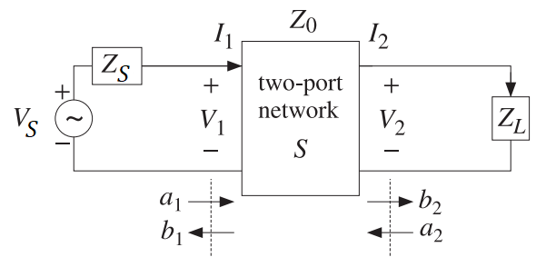
2-port network for transmission line S-parameters.
Here, we won’t make any other assumptions on the nature of the system other than we require the system to be causal and linear. There are some important points to consider in this general model as they will help us understand the general matrix equation for transmission line S-parameters.
- Unterminated line. The system shown above is assumed unterminated for the moment. Once we allow the line to be terminated, the equations above will reduce to the more familiar forms of the S-parameters and ABCD parameters. In this case, the S matrix shown above is not guranteed to be symmetric, thus the system is not reciprocal.
- Broadband. The S-parameters must be broadband parameters and obey Kramers-Kronig relations in order to satisfy causality in an LTI system. The Kramers-Kronig relations for the S-parameters could be derived manually, or we can apply this to the dielectric constant and regenerate the S-parameters using causal material parameters. We’ll take this latter approach as we’re working with a set of equations for S-parameters.
Now that we have the general model and assumptions for transmission line S-parameters, we have everything we need to describe the primary S-parameter matrix equation for this system. The S-parameter matrix is shown in the equation below in terms of ABCD parameters, which are defined directly from the general solution for any isolated transmission line (including with dielectric losses, copper roughness losses, and skin effect losses). Note that, if the system is not reciprocal, we may have different values for S11 and S22, as well as for S12 and S21. This is quite important as reflective behavior at each end of the line depends on the load impedance (determines S11 and S12) or on the driver’s impedance at the source end (determines S22 and S21).
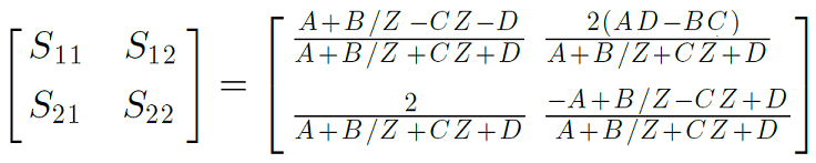
Primary matrix equation for transmission line S-parameters.
Note that there is an alternative expression with S-parameters that accounts for two different port impedances. This matrix equation is shown below. It is advised that the above equation be used for measurement (such as with a VNA), while the equation below be used for prediction with a real circuit:
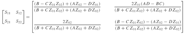
Matrix equation for transmission line S-parameters with unequal port impedances.
The form of this matrix may seem a bit complicated as Z in this equation is a reference impedance. You can choose this to be the load impedance if you like, although the line impedance is often used as this is more intuitive. Note that the conversion between different reference impedances is known as renormalization. The transmission line impedance doesn’t appear explicitly because it is lumped into the propagation constant for the transmission line and into the ABCD parameters. The ABCD parameters for any transmission line are defined below:
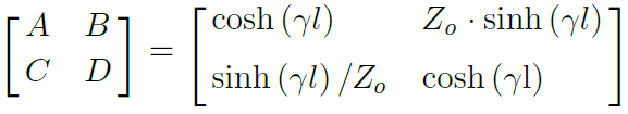
Primary matrix equation for transmission line ABCD-parameters.
If you ever want to convert your S-parameter measurements to ABCD parameters, you can use the following matrix equation:
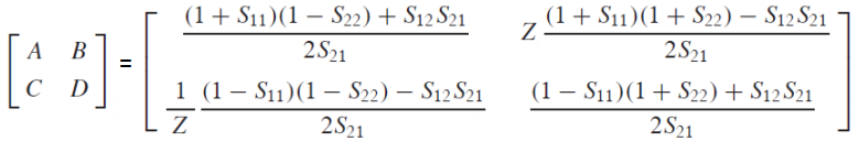
Conversion between transmission line S-parameters and ABCD parameters.
Transfer Function
Once you have the transmission line S-parameters or ABCD parameters, you can calculate a transfer function. This can be used to tell you how any signal will behave once it enters the transmission line and interacts with the load. The transfer function for the network can be calculated by converting the transmission line S-parameters to ABCD parameters, or vice versa (see above).
Note that the ABCD parameters are used to define the relationship between the input voltage/current and the output voltage/current. This direct calculation of inputs and outputs is not so important. Instead, we can lump these parameters into the transfer function. Given the ABCD parameters, we now have everything we need to determine the transfer function. The transfer function is defined in terms of ABCD parameters as shown below:
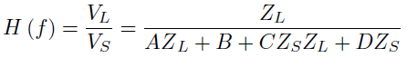
Transfer function for a transmission line using ABCD parameters.
Note that the transfer function is bandlimited, and it needs to be truncated using a windowing function. The signal travelling on the line is now a convolution of the input signal X(t) and the impulse response function h(t), where h(t) is truncated at t = 0 using the sign(x) function. Note that h(t) is the inverse Fourier transform of the transfer function that was found above:
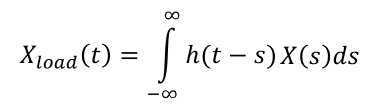
Convolution between the transfer function and input signal in the time domain.
Summary
In summary, we took the transmission line S-parameters and used them to calculate the signal behavior for an asymmetric transmission line. The general procedure can be summarized as follows:
- Select your input signal X(t)
- Calculate the Fourier transform of the input truncated at t = 0.
- Calculate the convolution in the frequency domain between the transfer function and FT[X(t)]
The resulting time-domain waveform shows you the signal reaching the load, which can be calculated as a function of the transmission line length. This tells you the signal seen at the receiver for any input signal X(t).
The design team at NWES specializes in high speed and high frequency board design, and we know how to extract and use your transmission line S-parameters to ensure signal integrity. We’re here to help electronics companies design modern PCB and create cutting-edge technology. We’re also a digital marketing firm, and we provide SEO-driven content marketing services for the products we design. We’re the best choice to market your product because we’ve built it and we’ve used it. Contact NWES for a consultation.
Ready to start your next design project?
Our Clients and Partners